[Model errors]  [Number of peaks]  [Peak width]  [Background correction]  [Random noise]  [Iterative fitting errors]  [Exponential broadening]  [Effect of smoothing]

Iterative curve fitting is often used to measure the position, height, and width of peaks in a signal, especially when they overlap significantly. There are four major sources of error in measuring these peak parameters by iterative curve fitting: model errors, background correction, random noise, and iterative fitting errors.  This section makes use of the downloadable peakfit.m function. Instructions are here or type "help peakfit". (Once you have peakfit.m in youjr path, you can simply copy and paste, or drag and drop, any of the following single-line or multi-line code examples into the Matlab or Octave editor or into the command line and press Enter to execute it).

a. Model errors. 
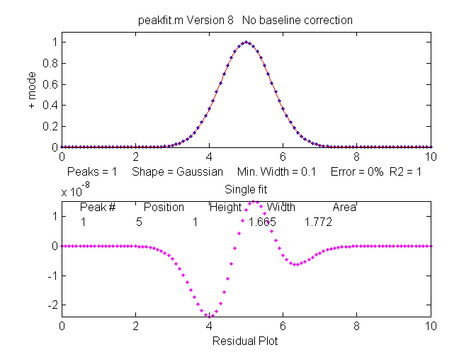
Peak shape. If you have the wrong model for your peaks, the results can not be expected to be accurate; for instance, if your actual peaks are Lorentzian in shape, but you fit them with a Gaussian model, or vice versa. For example, a single isolated Gaussian peak at x=5, with a height of 1.000 fits a Gaussian model virtually perfectly, using the Matlab user-defined peakfit function, as shown on the right. (The 5th input argument for the peakfit function specifies the shape of peaks to be used in the fit; "1" means Gaussian).

>> x=[0:.1:10];y=exp(-(x-5).^2);      
>> [FitResults,MeanFitError]=peakfit([x' y'],5,10,1,1)
Peak#     Position     Height      Width        Area
FitResults =
1            5            1       1.6651       1.7725
MeanFitError =         R2=
   7.8579e-07            1

The "FitResults" are, from left to right, peak number, peak position, peak height, peak width, and peak area. The MeanFitError, or just "fitting error", is the square root of  the sum of the squares of the differences between the data and the best-fit model, as a percentage of the maximum signal in the fitted region.  R2 is the "R-squared" or coefficient of determination, which is exactly 1 for a perfect fit. Note the good agreement of the area measurement (1.7725) with the theoretical area under the curve of exp(-x²), which turns out to be the square root of pi, or about 1.7725....

But this same peak, when fit with the incorrect model (a Logistic model, peak shape number 3), gives a fitting error of 1.4% and height and width errors of 3% and 6%, respectively. However, the peak area error is only 1.7%, because the height and width errors partially cancel out. So you don't have to have a perfect model to get a decent area measurement.

>> [FitResults,MeanFitError]=peakfit([x' y'],5,10,1,3)
Peak#     Position     Height      Width          Area
FitResults =
1       5.0002      0.96652        1.762       1.7419
MeanFitError =1.4095

When fit with an even more incorrect Lorentzian model (peak shape 2, shown on the right), this peak gives a 6% fitting error and height, width and area errors of 8%, 20%, and 17%, respectively.  

>> [FitResults,MeanFitError]=peakfit([x' y'],5,10,1,2)
FitResults =
Peak#     Position    Height      Width         Area
1            5       1.0876       1.3139       2.0579
MeanFitError =5.7893

But, practically speaking, Gaussian and Lorentzian shapes are so visually distinct that it's unlikely that your estimate of a model will be that far off. Real peak shapes are often some unknown combination of peak shapes, such as Gaussian with a little Lorentzian or vice versa, or some slightly asymmetrical modification of a standard symmetrical shape. So if you use an available model that is at least close to the actual shape, the parameters errors may not be so bad and may in fact be better than other measurement methods.

So clearly the larger the fitting errors, the larger are the parameter errors, but the parameter errors are of course not equal to the fitting error (that would just be too easy).  Also, it's clear that the peak height and width are the parameters most susceptible to errors. The peak positions, as you can see here, are measured accurately even if the model is way wrong, as long as the peak is symmetrical and not highly overlapping with other peaks. 

A good fit is not by itself proof that the shape function you have chosen is the correct one; in some cases the wrong function can give a fit that looks perfect. For example, this fit of a real data set to a 5-peak Gaussian model has a low percent fitting error and the residuals look random - usually an indicator of a good fit. But in fact in this case the model is wrong; that data came from an experimental domain where the underlying shape is fundamentally non-Gaussian but in some cases can look very like a Gaussian. As another example, a data set consisting of peaks with a Voigt profile peak shape can be fit with a  weighted sum of a Gaussian and a Lorentzian almost as well as an with an actual Voigt model, even though those models are not the same mathematically; the difference in fitting error is so small that it would likely be obscured by the random noise if it were a real experimental signal. The same thing can occur in sigmoidal signal shapes: a pair of simple 2-parameter logistic functions seems to fit this example data pretty well, with a fitting error of less than 1%; you would have no reason to doubt the goodness of fit unless the random noise is low enough so you can see that the residuals are wavy. Alternatively, a 3-parameter logistic (Gompertz function) fits much better, and the residuals are random, not wavy. In such cases you can not depend solely on what looks like a good fit to determine whether the fit is model is optimum; sometimes you need to know more about the peak shape expected in that kind of experiment, especially if the data are noisy. At best, if you do get a good fit with random non-wavy residuals, you can claim that the data are consistent with the proposed model. Note: with the peakfit.m function, you can extract the residuals as a vector by using the syntax [FitResults,GOF,baseline,coeff,residual,xi,yi]=peakfit(....

Sometimes the accuracy of the model is not so important. In quantitative analysis applications, where the peak height or areas measured by curve fitting is used only to determine the concentration of the substance that created the peak by constructing a calibration curve, using laboratory prepared standards solutions of known concentrations, the necessity of using the exact peak model is lessened, as long as the shape of the unknown peak is constant and independent of concentration. If the wrong model shape is used, the R² for curve fitting will be poor (much less than 1.000) and the peak heights and areas measured by curve fitting will be inaccurate, but the error will be exactly the same for the unknown samples and the known calibration standards, so the error will cancel out and, as a result, the R² for the calibration curve can be very high (0.9999 or better) and the measured concentrations will be no less accurate than they would have been with a perfect peak shape model. Even so, it's useful to use as accurate a model peak shape as possible, because the R² for curve fitting will work better as a warning indicator if something unexpected goes wrong during the analysis (such as an increase in the noise or the appearance of an interfering peak from a foreign substance). See PeakShapeAnalyticalCurve.m for a Matlab/Octave demonstration.

Number of peaks. Another source of model error occurs if you have the wrong number of peaks in your model, for example if the signal actually has two peaks but you try to fit it with only one peak. In the example below, a line of Matlab code generates a simulated signal with of two Gaussian peaks at x=4 and x=6 with peaks heights of 1.000 and 0.5000 respectively and widths of 1.665, plus random noise with a standard deviation 5% of the height of the largest peak (a signal-to-noise ratio of 20):

>>x=[0:.1:10];y=exp(-(x-6).^2)+.5*exp(-(x-4).^2)+.05*randn(size(x));

In a real experiment you would not usually know the peak positions, heights, and widths; you would be using curve fitting to measure those parameters. Let's assume that, on the basis of previous experience or some preliminary trial fits, you have established that the optimum peak shape model is Gaussian, but you don't know for sure how many peaks are in this group. If you start out by fitting this signal with a single-peak Gaussian model, you get:

>> [FitResults,MeanFitError]=peakfit([x' y'],5,10,1,1)

FitResults
   Peak#   Position   Height     Width      Area
   1       5.5291     0.86396    2.9789    2.7392
MeanFitError = 10.467

The residual plot shows a "wavy" structure that's visible in the random scatter of points due to the random noise in the signal. This means that the fitting error is not limited by the random noise; it is a clue that the model is not quite right. 

But a fit with two peaks yields much better results (The 4^th input argument for the peakfit function specifies the number of peaks to be used in the fit).

>> [FitResults,MeanFitError]=peakfit([x' y'],5,10,2,1)
FitResults =
      Peak#    Position  Height    Width    Area
       1      4.0165     0.50484   1.6982   0.91267
       2      5.9932     1.0018    1.6652   1.7759
MeanFitError =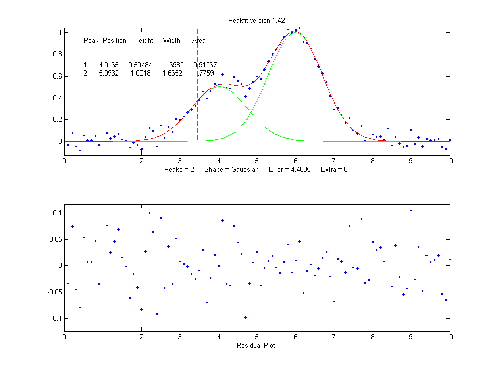 4.4635

Now the residuals have a random scatter of points, as would be expected if the signal is accurately fit except for the random noise. Moreover, the fitting error is much lower (less that half) of the error with only one peak. In fact, the fitting error is just about what we would expect in this case based on the 5% random noise in the signal (estimating the relative standard deviation of the points in the baseline visible at the edges of the signal). Because this is a simulation in which we know beforehand the true values of the peak parameters (peaks at x=4 and x=6 with peaks heights of 1.0 and 0.50 respectively and widths of 1.665), we can actually calculate the parameter errors (the difference between the real peak positions, heights, and widths and the measured values). Note that they are quite accurate (in this case within about 1% relative on the peak height and 2% on the widths), which is actually better than the 5% random noise in this signal because of the averaging effect of fitting to multiple data points in the signal. 

But if going from one peak to two peaks gave us a better fit, why not go to three peaks?  If there were no noise in the data, and if the underlying peak shape were perfectly matched by the model, then the fitting error would have already been essentially zero with two model peaks, and adding a third peak to the model would yield a vanishingly small height for that third peak. But in our examples here, as in real data, there is always some random noise, and the result is that the third peak height will not be zero. Changing the number of peaks to three gives these results:

>> [FitResults,MeanFitError]=peakfit([x' y'],5,10,3,1)
FitResults =
          Peak#  Position   Height    Width     Area
            1    4.0748     0.51617   1.7874    0.98212
            2    6.7799     0.089595  2.0455    0.19507
            3    5.9711     0.94455   1.53      1.5384
MeanFitError =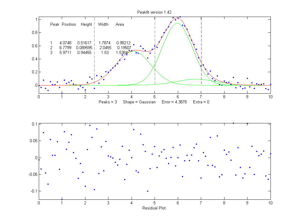 4.3878

The fitting algorithm has now tried to fit an additional low-amplitude peak (numbered peak 2 in this case) located at x=6.78. The fitting error is actually lower that for the 2-peak fit, but only slightly lower, and the residuals are no less visually random that with a 2-peak fit.  So, knowing nothing else, a 3-peak fit might be rejected on that basis alone. In fact, there is a serious downside to fitting more peaks than are actually present in the signal: it increases the parameter measurement errors of the peaks that are actually present. Again, we can prove this because we know beforehand the true values of the peak parameters: clearly the peak positions, heights, and widths of the two real peaks than are actually in the signal (peaks 1 and 3) are significantly less accurate than those of the 2-peak fit. 

Moreover, if we repeat that fit with the same signal but with a different sample of random noise (simulating a repeat measurement of a stable experimental signal in the presence or random noise), the additional third peak in the 3-peak fit will bounce around all over the place (because the third peak is actually fitting the random noise, not an actual peak in the signal). 

>> x=[0:.1:10];
>> y=exp(-(x-6).^2)+.5*exp(-(x-4).^2)+.05*randn(size(x));
>> [FitResults,MeanFitError]=peakfit([x' y'],5,10,3,1)
FitResults =
        Peak#   Position    Height     Width      Area
        1       4.115      0.44767     1.8768     0.89442
        2       5.3118     0.09340     2.6986     0.26832
        3       6.0681     0.91085     1.5116     1.4657
MeanFitError = 4.4089

With this new set of data, two of the peaks (numbers 1 and 3) have roughly the same position, height, and width, but peak number 2 has changed substantially compared to the previous run. Now we have an even more compelling reason to reject the 3-peak model: the 3-peak solution is not stable. And because this is a simulation in which we know the right answers, we can verify that the accuracy of the peak heights is substantially poorer (about 10% error) than expected with this level of random noise in the signal (5%). If we were to run a 2-peak fit on the same new data, we get much better measurements of the peak heights.

>> [FitResults,MeanFitError]=peakfit([x' y'],5,10,2,1)
FitResults =
         Peak#   Position    Height     Width     Area
          1      4.1601      0.49981    1.9108    1.0167
          2      6.0585      0.97557    1.548     1.6076
MeanFitError = 4.4113

If this is repeated several times, it turns out that the peak parameters of the peaks at x=4 and x=6 are, on average, more accurately measured by the 2-peak fit. In practice, the best way to evaluate a proposed fitting model is to fit several repeat measurements of the same signal (if that is practical experimentally) and to compute the standard deviation of the peak parameter values.

In real experimental work, of course, you usually don't know the right answers beforehand, so that's why it's important to use methods that work well when you do know. The real data example mentioned above was fit with a succession of 2, 3, 4 and 5 Gaussian models, until the residuals became random. Beyond that point, there is little to be gained by adding more peaks to the model. Another way to determine the minimum number of models peaks needed is to plot the fitting error vs the number of model peaks; the point at which the fitting error reaches a minimum, and increases afterward, would be the fit with the "ideal combination of having the best fit without excess/unnecessary terms". The Matlab/Octave function testnumpeaks.m (R = testnumpeaks(x, y, peakshape, extra, NumTrials, MaxPeaks)) applies this idea by fitting the x,y data to a series of models of shape peakshape containing 1 to MaxPeaks model peaks. The correct number of underlying peaks is either the model with the lowest fitting error, or, if two or more models have about the same fitting error, the model with the least number of peaks. The Matlab/Octave demo script NumPeaksTest.m uses this function with noisy computer-generated signals containing a user-selected 3, 4, 5 or 6 underlying peaks. With very noisy data, however, the technique is not always reliable.

Peak width constraints. Finally, there is one more thing that we can do that might improve the peak parameter measurement accuracy, and it concerns the peak widths. In all the above simulations, the basic assumption that all the peak parameters were unknown and independent of one another. In some types of measurements, however, the peak widths of each group of adjacent peaks are all expected to be equal to each other, on the basis of first principles or previous experiments. This is a common situation in analytical chemistry, especially in atomic spectroscopy and in chromatography, where the peak widths are determined largely by instrumental factors.

In the current simulation, the true peaks widths are in fact both equal to 1.665, but all the results above show that the measured peak widths are close but not quite equal, due to random noise in the signal. The unequal peak widths are a consequence of the random noise, not real differences in peak width. But we can introduce an equal-width constraint into the fit by using peak shape 6 (Equal-width Gaussians) or peak shape 7 (Equal-width Lorentzians). Using peak shape 6 on the same set of data as the previous example:

>> [FitResults,MeanFitError]=peakfit([x' y'],5,10,2,6)
FitResults =
           Peak#  Position   Height    Width    Area
            1     4.0293     0.52818   1.5666   0.8808
            2     5.9965     1.0192    1.5666   1.6997
MeanFitError =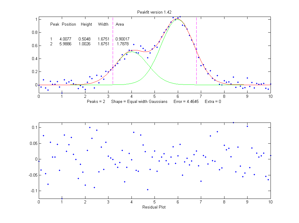 4.5588

This "equal width" fit forces all the peaks within one group to have exactly the same width, but that width is determined by the program from the data. The result is a slightly higher fitting error (in this case 4.5% rather than 4.4%), but - perhaps surprisingly - the peak parameter measurements are usually more accurate and more reproducible (Specifically, the relative standard deviations are on average lower for the equal-width fit than for an unconstrained-width fit to the same data, assuming of course that the true underlying peak widths are really equal). This is an exception to the general expectation that lower fitting errors result in lower peak parameter errors. It is an illustration of the general rule that the more you know about the nature of your signals, and the closer your chosen model adheres to that knowledge, the better the results. In this case we knew that the peak shape was Gaussian (although we could have verified that choice by trying other candidate peaks shapes). We determined that the number of peaks was 2 by inspecting the residuals and fitting errors for 1, 2, and 3 peak models. And then we introduced the constraint of equal peak widths within each group of peaks, based on prior knowledge of the experiment rather than on inspection of residuals and fitting errors. Here's another example, with real experimental data from a measurement where the peak widths are expected to be equal, showing the result of an unconstrained fit and an equal width fit; the fitting errors is slightly larger for the equal-width fit, but that is to be preferred in this case. Not every experiment can be expected to yield peaks of equal width, but when it does, it's better to make use of that constraint.  

Fixed-width shapes. Going one step beyond equal widths (in peakfit version 7.6 and later), you can also specify a fixed-width shapes (shape numbers 11, 12, 34-37), in which the width of the peaks are known beforehand, but are not necessarily equal, and are specified as a vector in input argument 10, one element for each peak, rather than being determined from the data as in the equal-width fit above. Introducing this constraint onto the previous example, and supplying an accurate width as the 10th input argument:  

>> [FitResults,MeanFitError]=peakfit([x' y'],0,0,2,11,0,0,0,0,[1.666 1.666])
FitResults =
        Peak#     Position     Height      Width       Area
          1       3.9943      0.49537      1.666      0.8785
          2       5.9924      0.98612      1.666      1.7488
MeanFitError = 4.8128

Comparing to the previous equal-width fit, the fitting error of 4.8% is larger here (because there are fewer degrees of freedom to minimize the error), but the parameter errors, particularly the peaks heights, are more accurate because the width information provided in the input argument was more accurate (1.666) than the width determined by the equal-width fit (1.5666). Again, not every experiment yields peaks of known width, but when it does, it's better to make use of that constraint. For example, see Example 35 and the Matlab/Octave script WidthTest.m (typical results for a Gaussian/Lorentzian blend shape shown below, showing that the more constraints, the greater the fitting error but the lower the parameter errors, if the constraints are accurate).

Relative percent error	Fitting error	Position Error	Height Error	Width Error
Unconstrained shape factor and widths: shape 33	0.78	0.39	0.80	1.66
Fixed shape factor and variable widths: shape 13	0.79	0.25	1.3	0.98
Fixed shape factor and fixed widths: shape 35	0.8	0.19	0.69	0.0

Multiple linear regression (peakfit version 9). Finally, note that if the peak positions are also known, and only the peak heights are unknown, you don't even need to use the iterative fitting method at all; you can use the easier and faster multilinear regression technique (also called "classical least squares") which is implemented by the function cls.m and by version 9 of peakfit.m as shape number 50. Although multilinear regression results in fitting error slightly greater (and R2 lower), the errors in the measured peak heights are often less, as in this example from peakfit9demo.m, where the true peak heights of the three overlapping Gaussian peaks are 10, 30, and 20. 
 Multilinear regression results (known position and width):
           Peak    Position     Height       Width   Area
            1         400      9.9073         70     738.22
            2         500      29.995         85     2714
            3         560      19.932         90     1909.5
%fitting error=1.3048   R2= 0.99832   %MeanHeightError=0.427

Unconstrained iterative non-linear least squares results:
           Peak   Position     Height      Width    Area
            1      399.7      9.7737      70.234    730.7
            2      503.12     32.262      88.217    3029.6
            3      565.08     17.381      86.58     1601.9
%fitting error=1.3008   R2= 0.99833   %MeanHeightError=7.63
This demonstrates dramatically how different measurement methods can look the same, and give fitting errors almost the same, and yet differ greatly in parameter measurement accuracy. (The similar script peakfit9demoL.m is the same thing with Lorentzian peaks).

SmallPeak.m is a demonstration script comparing all these techniques applied to the challenging problem of measuring the height of a small peak that is closely overlapped with and completely obscured by a much larger peak. It compares unconstrained, equal-width, and fixed-position iterative fits (using peakfit.m) with a classical least squares fit in which only the peak heights are unknown (using cls.m). It helps to spread out the four figure windows so you can observe the dramatic difference in stability of the different methods. A final table of relative percent peak height errors shows that the more the constraints, the better the results (but only if the constraints are justified). The real key is to know which parameters can be relied upon to be constant and which have to be allowed to vary.

Here's a a screen video (MorePeaksLowerFittingError.mp4) of a real-data experiment using the interactive peak fitter ipf.m with a complex experimental signal in which several different fits were performed using models from 4 to 9 variable-width, equal-width, and fixed-width Gaussian peaks. The fitting error gradually decreases from 11% initially to 1.4% as more peaks are used, but is that really justified? If the objective is simply to get a good fit, then do whatever it takes. But if the objective is to extract some useful information from the model peak parameters, then more specific knowledge about that particular experiment is needed: how many peaks are really expected; are the peak widths really expected to be constrained? Note that in this particular case the residuals (bottom panel) are never really random and always have a distinct "wavy" character, suggesting that the data may have been smoothed before curve fitting (usually not a good idea: see http://wmbriggs.com/blog/?p=195). Thus there is a real possibility that some of those 9 peaks are simply "fitting the noise", as will be discussed further in Appendix A.

b. Background correction.
The peaks that are measured in many scientific instruments are sometimes superimposed on a non-specific background or baseline. Ordinarily the experiment protocol is designed to minimize the background or to compensate for the background, for example by subtracting a "blank" signal from the signal of an actual specimen. But even so there is often a residual background that can not be eliminated completely experimentally. The origin and shape of that background depends on the specific measurement method, but often this background is a broad, tilted, or curved shape, and the peaks of interest are comparatively narrow features superimposed on that background. In some cases the baseline may be another peak. The presence of the background has relatively little effect on the peak positions, but it is impossible to measure the peak heights, width, and areas accurately unless something is done to account for the background.

There are various methods described in the literature for estimating and subtracting the background in such cases. The simplest assumption is that the background can be approximated as a simple function in the local region of group of peaks being fit together, for example as a constant (flat), straight line (linear) or curved line (quadratic). This is the basis of the "autozero" modes in the ipf.m, iSignal.m, and iPeak.m functions, which are selected by the T key to cycle thorough OFF, linear, quadratic, and flat modes. In the flat mode, a constant baseline is included in the curve fitting calculation, as described above. In linear mode, a straight-line baseline connecting the two ends of the signal segment in the upper panel will be automatically subtracted before the iterative curve fitting. In quadratic mode, a parabolic baseline is subtracted. In the last two modes, you must adjust the pan and zoom controls to isolate the group of overlapping peaks to be fit, so that the signal returns to the local background at the left and right ends of the window.

Example of an experimental chromatographic signal. From left to right, (1) Raw data with peaks superimposed on a tilted baseline. One group of peaks is selected using the the pan and zoom controls, adjusted so that the signal returns to the local background at the edges of the segment displayed in the upper window; (2) The linear baseline is subtracted when the autozero mode set to 1 in ipf.m by pressing the T key; (3) Fit with a three-peak Gaussian model, activated by pressing 3, G, F (3 peaks, Gaussian, Fit).

Alternatively, it may be better to subtract the background from the entire signal first, before further operations are performed. As before, the simplest assumption is that the background is piece-wise linear, that is, can be approximated as a series of small straight line segments.  This is the basis of the multiple point background subtraction mode in ipf.m, iPeak.m, and in iSignal. The user enters the number of points that is thought to be sufficient to define the baseline, then clicks where the baseline is thought to be along the entire length of the signal in the lower whole-signal display (e.g. on the valleys between the peaks).  After the last point is clicked, the program interpolates between the clicked points and subtracts the piece-wise linear background from the original signal.

  From left to right, (1) Raw data with peaks superimposed on baseline. (2) Background subtracted from the entire signal using the multipoint background subtraction function in iPeak.m (ipf.m and iSignal have the same function).

Sometimes, even without an actual baseline present, the peaks may overlap enough so that the signal never return to the baseline, making it seem that there is a baseline to be corrected. This can occur especially with peaks shapes that have gradually sloping sides, such as the Lorentzian, as shown in this example. Curve fitting without baseline correction will work in that case.

In many cases the background may be modeled as a broad peak whose maximum falls outside of the range of data acquired, as in the real-data example on the left. It may be possible to fit the off-screen peak simply by including an extra peak in the model to account for the baseline. In the example on the left, there are three clear peaks visible, superimposed on a tilted baseline. In  this case the signal was fit nicely with four, rather than three, variable-width Gaussians, with an error of only 1.3%. The additional broad Gaussian, with a peak at  x = -38.7, serves as the baseline. (Obviously, you shouldn't use the equal-width shapes for this, because the background peak is broader than the other peaks).

In another real-data example of an experimental spectrum, the linear baseline subtraction ("autozero") mode described above is used in conjunction with a 5-Gaussian model, with one Gaussian component fitting the broad peak that may be part of the background and the other four fitting the sharper peaks. This fits the data very well (0.5% fitting error), but a fit like this can be difficult to get, because there are so many other solutions with slightly higher fitting errors; it may take several trials. It can help if you specify the start values for the iterated variables, rather than using the default choices; all the software programs described here have that capability.

The Matlab/Octave function peakfit.m can employ a peakshape input argument that is a vector of different shapes, which can be useful for baseline correction. As an example, consider a weak Gaussian peak on sloped straight-line baseline, using a 2-component fit with one Gaussian component and one variable-slope straight line ('slope', shape 26), specified by using the vector [1 26] as the shape argument:

x=8:.05:12;y=x+exp(-(x-10).^2);
[FitResults,GOF]= peakfit([x;y],0,0,2,[1 26],[1 1],1,0)
FitResults =          
    1         10          1     1.6651     1.7642
    2      4.485    0.22297       0.05     40.045
GOF =
    0.0928    0.9999

If the baseline seems to be curved rather than straight, you can model the baseline with a quadratic (shape 46) rather than a linear slope (peakfit version 8 and later).

If the baseline seems to be different on either side of the peak, you can try to model the baseline with an S-shape (sigmoid), either an up-sigmoid, shape 10 (click for graphic), peakfit([x;y],0,0,2,[1 10],[0 0], or a down-sigmoid, shape 23 (click for graphic), peakfit([x;y],0,0,2,[1 23],[0 0], in these examples leaving the peak modeled as a Gaussian.

If the signal is very weak compared to the baseline, the fit can be helped by adding rough first guesses ('start') using the 'polyfit' function to generate automatic first guesses for the sloping baseline. For example, with two overlapping signal peaks and a 3-peak fit with peakshape=[1 1 26].

x=4:.05:16;
y=x+exp(-(x-9).^2)+exp(-(x-11).^2)+.02.*randn(size(x));
start=[8 1 10 1 polyfit(x,y,1)];
peakfit([x;y],0,0,3,[1 1 26],[1 1 1],1,start)

        A similar technique can be employed in a spreadsheet, as demonstrated in CurveFitter2GaussianBaseline.xlsx (graphic).

The downside to including the baseline as a variable component is that it increases the number of degrees of freedom, increases the execution time, and increases the possibility of unstable fits. Specifying start values can help.

c. Random noise in the signal. 
Any experimental signal has a certain amount of random noise, which means that the individual data points scatter randomly above and below their mean values.  The assumption is ordinarily made that the scatter is equally above and below the true signal, so that the long-term average approaches the true mean value; the noise "averages to zero" as it is often said. The practical problem is that any given recording of the signal contains only one finite sample of the noise.  If another recording of the signal is made, it will contain another independent sample of the noise. These noise samples are not infinitely long and therefore do not represent the true long-term nature of the noise. This presents two problems: (1) an individual sample of the noise will not "average to zero" and thus the  parameters of the best-fit model will not necessarily equal the true values, and (2) the magnitude of the noise during one sample might not be typical; the noise might have been randomly greater or smaller than average during that time. This means that the mathematical "propagation of error" methods, which seek to estimate the likely error in the model parameters based on the noise in the signal, will be subject to error (underestimating the error if the noise happens to be lower than average and overestimating the errors if the noise happens to be larger than average).

A better way to estimate the parameter errors is to record multiple samples of the signal, fit each of those separately, compute the models parameters from each fit, and calculate the standard error of each parameter. But if that is not practical, it is possible to simulate such measurements by adding random noise to a model with known parameters, then fitting that simulated noisy signal to determine the parameters, then repeating the procedure over and over again with different sets of random noise. This is exactly what the script DemoPeakfit.m (which requires the peakfit.m function) does for simulated noisy peak signals such as those illustrated below. It's easy to demonstrate that, as expected, the average fitting error precision and the relative standard deviation of the parameters increases directly with the random noise level in the signal. But the precision and the accuracy of the measured parameters also depend on which parameter it is (peak positions are always measured more accurately than their heights, widths, and areas) and on the peak height and extent of peak overlap (the two left-most peaks in this example are not only weaker but also more overlapped than the right-most peak, and therefore exhibit poorer parameter measurements). In this example, the fitting error is 1.6% and the percent relative standard deviation of the parameters ranges from 0.05% for the peak position of the largest peak to 12% for the peak area of the smallest peak.

  

Overlap matters: The errors in the values of peak parameters measured by curve fitting depend not only on the characteristics of the peaks in question and the signal-to-noise ratio, but also upon other peaks that are overlapping it.  From left to right: (1) a single peak at x=100 with a peak height of 1.0 and width of 30 is fit with a Gaussian model, yielding a relative fit error of 4.9% and relative standard deviation of peak position, height, and width of  0.2%, 0.95%, and 1.5% , respectively. (2) The same peak, with the same noise level but with another peak overlapping it, reduces the relative fit error to 2.4% (because the addition of the second peak increases overall signal amplitude), but increases the relative standard deviation of peak position, height, and width to 0.84%, 5%, and 4% - a seemingly better fit, but with poorer precision for the first peak. (3) The addition of a third (non-overlapping) peak reduces the fit error to 1.6% , but the relative standard deviation of peak position, height, and width of the first peak are still 0.8%, 5.8%, and 3.64%, about the same as with two peaks, because the third peak does not overlap the first one significantly.

If the average noise noise in the signal is not known or its probability distribution is uncertain, it is possible to use the bootstrap sampling method to estimate the uncertainty of the peak heights, positions, and widths, as illustated on the left and as described in detail above. The latest version of the keypress operated interactive version of ipf.m has added a function (activated by the 'v' key) that estimates the expected standard deviation of the peak parameters using this method. 

One way to reduce the effect of noise is to take more data. If the experiment makes it possible to reduce the x-axis interval between points, or to take multiple readings at each x-axis values, then the resulting increase in the number of data points in each peak should help reduce the effect of noise. As a demonstration, using the script DemoPeakfit.m to create a simulated overlapping peak signal like that shown above right, it's possible to change the interval between x values and thus the total number of data points in the signal. With a noise level of 1% and 75 points in the signal, the fitting error is 0.35 and the average parameter error is 0.8%. With 300 points in the signal and the same noise level, the fitting error is essentially the same, but the average parameter error drops to 0.4%, suggesting that the accuracy of the measured parameters varies inversely with the square root of the number of data points in the peaks.

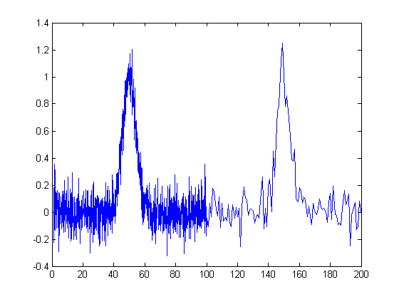The figure on the right illustrates the importance of sampling interval and data density. You can download the data file "udx" in TXT format or in Matlab MAT format. The signal consists of two Gaussian peaks, one located at x=50 and the second at x=150. Both peaks have a peak height of 1.0 and a peak half-width of 10, and normally-distributed random white noise with a standard deviation of 0.1 has been added to the entire signal. The x-axis sampling interval, however, is different for the two peaks; it's 0.1 for the first peak and 1.0 for the second peak. This means that the first peak is characterized by ten times more points than the second peak. When you fit these peaks separately to a Gaussian model (e.g., using peakfit.m or ipf.m), you will find that all the parameters of the first peak are measured more accurately than the second, even though the fitting error is not much different:

First peak:                                                      Second peak:
Percent Fitting Error=7.6434%  Percent Fitting Error=8.8827%
Peak# Position Height Width    Peak# Position  Height  Width
1      49.95   1.0049 10.111   1     149.64   1.0313   9.941

So far this discussion has applied to white noise. But other noise colors have different effects. Low-frequency weighted ("pink") noise has a greater effect on the accuracy of peak parameters measured by curve fitting, and, in a nice symmetry, high-frequency "blue" noise has a smaller effect on the accuracy of peak parameters that would be expected on the basis of its standard deviation, because the information in a smooth peak signal is concentrated at low frequencies. An example of this occurs when curve fitting is applied to a signal that has been deconvoluted to remove a broadening effect. This is why smoothing before curve fitting does not help, because the peak signal information is concentrated in the low frequency range, but smoothing reduces mainly the noise in the high frequency range.

Sometime you may notice that the residuals in a curve fitting operation are structured into bands or lines rather than being completely random. This can occur if either the independent variable or the dependent variable is quantized into discrete steps rather than continuous. It may look strange, but it has little effect on the results as long as the random noise is larger than the steps.

When there is noise in the data (in other words, pretty much always), the exact results will depend on the region selected for the fit - for example, the results will vary slightly with the pan and zoom setting in ipf.m, and the more noise, the greater the effect.

d. Iterative fitting errors.
Unlike multiple linear regression curve fitting, iterative methods may not always converge on the exact same model parameters each time the fit is repeated with slightly different starting values (first guesses). The Interactive Peak Fitter ipf.m makes it easy to test this, because it uses slightly different starting values each time the signal is fit (by pressing the F key in ipf.m, for example). Even better, by pressing the X key, the ipf.m function silently computes 10 fits with different starting values and takes the one with the lowest fitting error. A basic assumption of any curve fitting operation is that the fitting error (the root-mean-square difference between the model and the data) is minimized, the parameter errors (the difference between the actual parameters and the  parameters of the best-fit model) will also be minimized. This is generally a good assumption, as demonstrated by the graph to the right, which shows typical percent parameters errors as a function of fitting error for the left-most peak in one sample of the simulated signal generated by DemoPeakfit.m (shown in the previous section). The variability of the fitting error here is caused by random small variations in the first guesses, rather than by random noise in the signal.  In many practical cases there is enough random noise in the signals that the iterative fitting errors within one sample of the signal are small compared to the random noise errors between samples. 

Remember that the variability in measured peak parameters from fit to fit of a single sample of the signal is not a good estimate of the precision or accuracy of those parameters, for the simple reason that those results represent only one sample of the signal, noise, and background. The sample-to-sample variations are likely to be much greater than the within-sample variations due to the iterative curve fitting. (In this case, a "sample" is a single recording of signal). To estimate the contribution of random noise to the variability in measured peak parameters when only a single sample if the signal is available, the bootstrap method can be used.

e. Selecting the optimum data region of interest.  When you perform a peak fitting using ipf.m, you have control over data region selected by using the pan and zoom controls (or, using the command-line function peakfit.m, by setting the center and window input arguments). Changing these settings usually changes the resulting fitted peak parameters. If the data were absolutely perfect, say, a mathematically perfect peak shape with no random noise, then the pan and zoom settings would make no difference at all; you would get the exact same values for peak parameters at all settings, assuming only that the model you are using matches the actual shape. But of course in the real world, data are never mathematically perfect and noiseless. The greater the amount of random noise in the data, or the greater the discrepancy between your data and the model you select, the more the measured parameters will vary if you fit different regions using the pan and zoom controls. This is simply an indication of the uncertainty in the measured parameters.

f. A difficult case. As a dramatic example of the ideas in parts c and d, consider 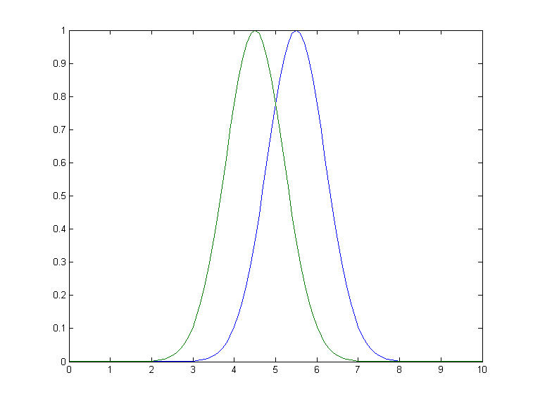this simulated example signal, consisting of two Gaussian peaks of equal height = 1.00, overlapping closely enough so that their sum is a single symmetrical peak that looks very much like a single Gaussian.

If there were no noise in the signal, the peakfit.m or ipf.m routines could easily extract the two equal Gaussian components to an accuracy of 1 part in 1000.

>> peakfit([x y],5,19,2,1)

          Peak#   Position   Height     Width    Area
           1      4.5004    1.001     1.6648    1.773
           2      5.5006    0.99934   1.6641    1.770

But in the presence of even a little noise (for example, 1% RSD), the results are uneven; one peak is almost always significantly higher than the other:

     Peak#   Position    Height     Width    Area
       1      4.4117     0.83282    1.61     1.43
       2      5.4022     1.1486     1.734    2.12

The fit is stable with any one sample of noise (if peakfit.m was run again with slightly different starting values, for example by pressing the F key several times in ipf.m), so the problem is not iterative fitting errors caused by different starting values. The problem is the noise: although the signal is completely symmetrical, any particular sample of the noise is not perfectly symmetrical (e.g. the first half of the noise usually averages a slightly higher or lower than the second half, resulting in an asymmetrical fit result). The surprising thing is that the error in the peak heights are much larger (about 15% relative, on average) than the random noise in the data (1% in this example). So even though the fit looks good - the fitting error is low (less than 1%) and the residuals are random and unstructured - the model parameters can still be very far off. If you were to make another measurement (i.e. generate another independent set of noise), the results would be different but still inaccurate (the first peak has an equal chance of being larger or smaller than the second). Unfortunately, the expected error is not accurately predicted by the bootstrap method, which seriously underestimates the standard deviation of the peak parameters with repeated measurements of independent signals (because a bootstrap sub-sample of asymmetrical noise is likely to remain asymmetrical). A Monte Carlo simulation would give a more reliable estimation of uncertainty in such cases. 

Better results can be obtained in cases where the peak widths are expected to be equal, in which case you can use peak shape 6 (equal-width Gaussian) instead of peak shape 1: peakfit([x y],5,19,2,6). It also helps to provide decent first guesses (start) and to set the number of trials (NumTrials) to a number above 1): peakfit([x,y],5,10,2,6,0,10,[4 2 5 2],0,0). The best case will be if the shape, position, and width of the two peaks are known accurately, and if the only unknown is their heights. Then the Classical Least Squares (multiple regression) technique can be employed and the results will be much better.

Appendix AE illustrates one way to deal with the problem of excessive peak overlap in a multi-step script that uses first-derivative symmetrization as a pre-process performed before iterative least-squares curve fitting to analyze a complex signal consisting of multiple asymmetric overlapping peaks. This results in better peak parameter accuracy, even though the fitting error is no better.

For an even more challenging example like this, where the two closely overlapping peak are very different in height, see Appendix Q.

So, to sum up, we can make the following observations about the accuracy of model parameters: (1) the parameter errors depend on the accuracy of the model chosen and on number of peaks; (2) the parameter errors are directly proportional to the noise in the data (and worse for low-frequency or pink noise); (3) all else being equal, parameter errors are proportional to the fitting error, but a model that fits the underlying reality better, e.g. equal or fixed widths or shapes) often gives lower parameter errors even if the fitting error is larger; (4) the errors are typically least for peak position and worse for peak width and area; (5) the errors depend on the data density (number of independent data points in the width of each peak) and on the extent of peak overlap (the parameters of isolated peaks are easier to measure than highly overlapped peaks); (6) if only a single signal is available, the effect of noise on the standard deviation of the peak parameters in many cases can be predicted approximately by the bootstrap method, but if the overlap of the peaks is too great, the error of the parameter measurements can be much greater than predicted.

  Fitting signals that are subject to exponential broadening.

DataMatrix2 (figure on the right) is a computer-generated test signal consisting of 16 symmetrical Gaussian peaks with random whi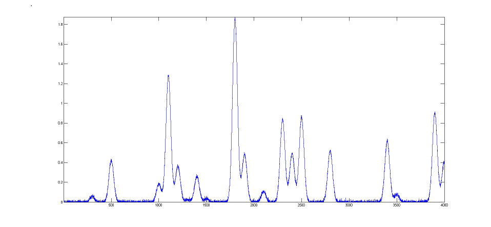te noise added. The peaks occur in groups of 1, 2, or 3 overlapping peaks, but the peak maxima are located at exactly integer values of x from 300 to 3900 (on the 100's) and the peak widths are always exactly 60 units. The peak heights vary from 0.06 to 1.85. The standard deviation of the noise is 0.01. You can use this signal to test curve-fitting programs and to determine the accuracy of their measurements of peak parameters. Right-click and select "Save" to download this signal, put it in the Matlab path, then type "load DataMatrix2" at the command prompt to load it into the Matlab workspace.

DataMatrix3 (figure on the left) i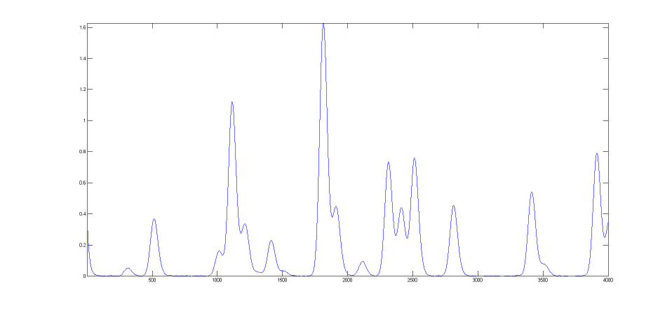s a exponentially broadened version of DataMatrix2, with a "decay constant", also called "time constant", of 33 points on the x-axis.  The result of the exponential broadening is that all the peaks in this signal are asymmetrical, their peak maxima are shifted to longer x values, and their peak heights are smaller and their peak widths are larger than the corresponding peaks in DataMatrix2. Also, the random noise is damped in this signal compared to the original and is no longer "white", as a consequence of the broadening. This type of effect is common in physical measurements and often arises from some physical or electrical effect in the measurement system that is apart from the fundamental peak characteristics. In such cases it is usually desirable to compensate for the effect of the broadening, either by deconvolution or by curve fitting, in an attempt to measure what the peak parameters would have been before the broadening (and also to measure the broadening itself).  This can be done for Gaussian peaks that are exponentially broadened by using the "ExpGaussian" peak shape in peakfit.m and ipf.m (or the "ExpLorentzian", if the underlying peaks are Lorentzian).  Right-click and select "Save" to download this signal, put it in the Matlab path, then type "load DataMatrix3" to load it into the Matlab workspace.

The example illustrated on the right focuses on the single isolated peak whose "true" peak position, height, width, and area in the original unbroadened signal, are 2800, 0.52, 60, and 33.2 respectively. (The relative standard deviation of the noise is 0.01/0.52=2%.) In the broadened signal, the peak is visibly asymmetrical, the peak maximum is shifted to larger x values, and it has a shorter height and larger width, as demonstrated by the attempt to fit a normal (symmetrical) Gaussian to the broadened peak. (The peak area, on the other hand, is  not much effected by the broadening). 

>> load DataMatrix3

>> ipf(DataMatrix3);

Peak Shape = Gaussian
Autozero ON
Number of peaks = 1
Fitted range = 2640 - 2979.5 (339.5)  (2809.75) 
Percent Error = 1.2084
Peak# Position  Height      Width      Area
1     2814.832  0.45100549  68.441262  32.859436

The large "wavy" residual in the plot above is a tip-off that the model is not quite right. Moreover, the fitting error (1.2%) is larger than expected for a peak with a half-width of 60 points and a 2% noise RSD (approximately 2%/sqrt(60)=0.25%).

Fitting to an exponentially-broadened Gaussian (pictured on the right) gives a much lower fitting error ("Percent error") and a more nearly random residual plot. But the interesting thing is that it also recovers the original peak position, height, and width to an accuracy of a fraction of 1%. In performing this fit, the decay constant ("extra") was experimentally determined from the broadened signal by adjusting it with the A and Z keys to give the lowest fitting error; that also results in a reasonably good measurement of the broadening factor (32.6, vs the actual value of 33). Of course, had the original signal been nosier, these measurements would not be so accurate. Note: When using peakshape 5 (fixed decay constant exponentially broadened Gaussian) you have to give it a reasonably good value for the  decay constant ('extra'), the input argument right after the peakshape number.  If the value is too far off, the fit may fail completely, returning all zeros. A little trial and error suffice. (Also, peakfit.m version 8.4 has two forms of unconstrained variable decay constant exponentially-broadened Gaussian, shape numbers 31 and 39, that will measure the decay constant as an iterated variable. Shape 31 (expgaussian.m) creates the shape by performing a Fourier convolution of a specified Gaussian by an exponential decay of specified decay constant, whereas shape 39 (expgaussian2.m) uses a mathematical expression for the final shape so produced. Both result in the same peak shape but are parameterized differently. Shape 31 reports the peak height and position as that of the original Gaussian before broadening, whereas shape 39 reports the peak height of the broadened result. Shape 31 reports the width as the FWHM (full width at half maximum) and shape 39 reports the standard deviation (sigma) of the Gaussian. Shape 31 reports the exponential factor an the number of data points and shape 39 reports the reciprocal of decay constant in time units. (See the script DemoExpgaussian.m for a more detailed numerical example). For multiple-peak fits, both shapes usually require a reasonable first guess ('start") vector for best results. If the exponential decay constant of each peak is expected to be different and you need to measure those values, use shapes 31 or 39, but the decay constant of all the peaks is expected to be the same, use shape 5, and determine the decay constant by fitting an isolated peak. For example:

Peak Shape = Exponentially-broadened Gaussian
Autozero ON
Number of peaks = 1
Extra = 32.6327
Fitted range = 2640 - 2979.5 (339.5)  (2809.75) 
Percent Error = 0.21696
Peak#  Position   Height      Width      Area
1      2800.1302  0.51829906  60.086295  33.152429

Comparing the two methods, the exponentially-broadened Gaussian fit recovers all the underlying peak parameters quite accurately:

	Position	Height	Width	Area
Actual peak parameters	2800	0.52	60	33.2155
Gaussian fit to broadened signal	2814.832	0.45100549	68.441262	32.859436
ExpGaussian fit to broadened signal	2800.1302	0.51829906	60.086295	33.152429

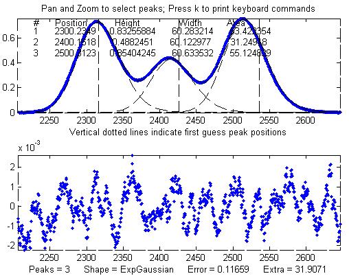Other peaks in the same signal, under the broadening influence of the same decay constant, can be fit with similar settings, for example the set of three overlapping peaks near x=2400.  As before, the peak positions are recovered almost exactly and even the width measurements are reasonably accurate (1% or better). If the exponential broadening decay constant is not the same for all the peaks in the signal, for example if it gradually increases for larger x values, then the decay constant setting can be optimized for each group of peaks. 

The smaller fitting error evident here is just a reflection of the larger peak heights in this particular group of peaks - the noise is the same everywhere in this signal.

Peak Shape = Exponentially-broadened Gaussian
Autozero OFF
Number of peaks = 3
Extra = 31.9071
Fitted range = 2206 - 2646.5 (440.5)  (2426.25) 
Percent Error = 0.11659
Peak# Position    Height      Width       Area
1     2300.2349  0.83255884   60.283214   53.422354
2     2400.1618  0.4882451    60.122977   31.24918
3     2500.3123  0.85404245   60.633532   55.124839

The residual plots in both of these examples still have some "wavy" character, rather than being completely random and "white".  The exponential broadening smooths out any white noise in the original signal that is introduced before the exponential effect, acting as a low-pass filter in the time domain and resulting in a low-frequency dominated "pink" noise, which is what remains in the residuals after the broadened peaks have been fit as well as possible. On the other hand, white noise that is introduced after the exponential effect would continue to appear white and random on the residuals.  In real experimental data, both types of noise may be present in varying amounts. 

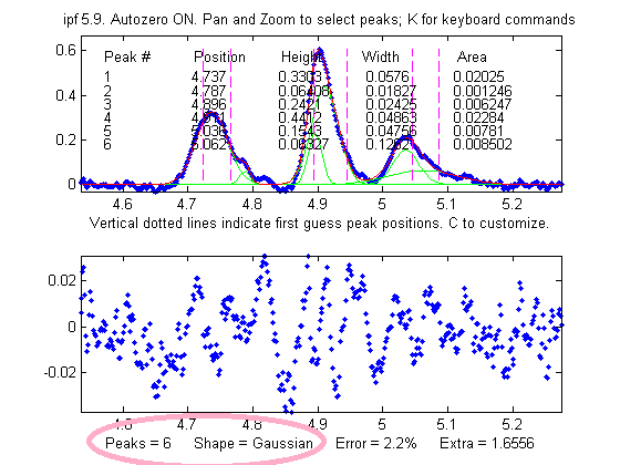
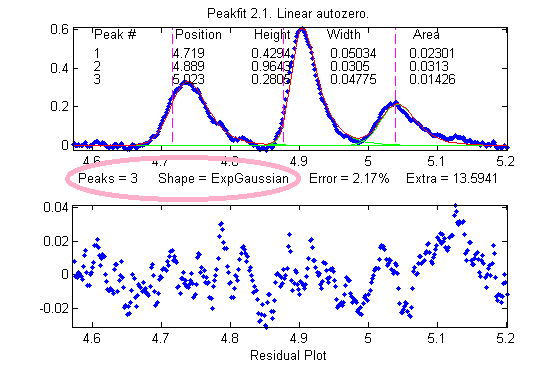One final caveat: peak asymmetry similar to exponential broadening could possibly be the result a pair of closely-spaced peaks of different peak heights.  In fact, a single exponential broadened Gaussian peak can sometimes be fit with two symmetrical Gaussians to a fitting error at least as low as a single exponential broadened Gaussian fit. This makes it hard to distinguish between these two models on the basis of fitting error alone. However, this can usually be decided by inspecting the other peaks in the signal: in most experiments, exponential broadening applies to every peak in the signal, and the broadening is either constant or changes gradually over the length of the signal. On the other hand, it is relatively unlikely that every peak in the signal will be accompanied by a smaller side peak that varies in this way. So, if a only one or a few of the peaks exhibit asymmetry, and the others are symmetrical, it's most likely that the asymmetry is due to closely-spaced peaks of different peak heights. If all peaks have the same or similar asymmetry, it's more likely to be a broadening factor that applies to the entire signal. The two figures here provide an example from real experimental data. On the left, three asymmetrical peaks are each fit with two symmetrical Gaussians (six peaks total). On the right, those three peaks are fit with one exponentially broadened Gaussian each (three peaks total). In this case, the three asymmetrical peaks all have the same asymmetry and can be fit with the same decay constant ("extra"). Moreover, the fitting error is slightly lower for the three-peak exponentially broadened fit. Both of these observations argue for the three-peak exponentially broadened fit rather than the six-peak fit.

Note: if your peaks are trailing off to the left, rather that to the right as in the above examples, simply use a negative value for the decay constant (in ipf.n, press Shift-X and type a negative values).

An alternative to this type of curve fitting for exponential broadened peaks is to use the first-derivative addition technique to remove the asymmetry and then fit the resulting peak with a symmetrical model. This is faster in terms of computer execution time, especially for signals with many peaks, but it requires that the exponential time constant be known or estimated experimentally beforehand. 

The Effect of Smoothing before least-squares analysis.

In general, it is not advisable to smooth a signal before applying least-squares fitting, because doing so might distort the signal, can make it hard to evaluate the residuals properly, and might bias the results of bootstrap sampling estimations of precision, causing it to underestimate the between-signal variations in peak parameters. SmoothOptimization.m is a Matlab/Octave script that compares the effect of smoothing on the measurements of peak height of a Gaussian peak with a half-width of 166 points, plus white noise with a signal-to-noise ratio (SNR) of 10, using three different methods:
  (a) simply taking the single point at the center of the peak as the peak height;
  (b) using the gaussfit method to fit the top half of the peak (see CurveFitting.html#Transforming), and
  (c) fitting the entire signal with a Gaussian using the iterative method.
The results of 150 trials with independent white noise samples are shown on the left: a typical raw signal is shown in the upper left. The other three plots show the effect of the SNR of the measured peak height vs the smooth ratio (the ratio of the smooth width to the half-width of the peak) for those three measurement methods. The results show that the simple single-point measurement is indeed much improved by smoothing, as is expected; however, the optimum SNR (which improves by roughly the square root of the peak width of 166 points) is achieved only when the smooth ratio approaches 1.0, and that much smoothing distorts the peak shape significantly, reducing the peak height by about 40%. The curve-fitting methods are much less effected by smoothing and the iterative method hardly at all. So the bottom line is that you should not smooth prior to curve-fitting, because it will distort the peak and will not gain any significant SNR advantage. The only situations where it might be advantageous so smooth before fitting are when the noise in the signal is high-frequency weighted (i.e. "blue" noise), where low-pass filtering will make the peaks easier to see for the purpose of setting the staring points for an iterative fit, or if the signal is contaminated with high-amplitude narrow spike artifacts, in which case a median-based pre-filter can remove the spikes without much change to the rest of the signal. And, in another application altogether, if you want to fit a curve joining the successive peaks of a modulated wave (called the "envelope"), then you can smooth the absolute value of the wave before fitting the envelope.
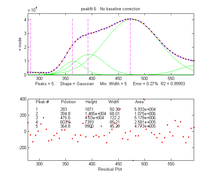
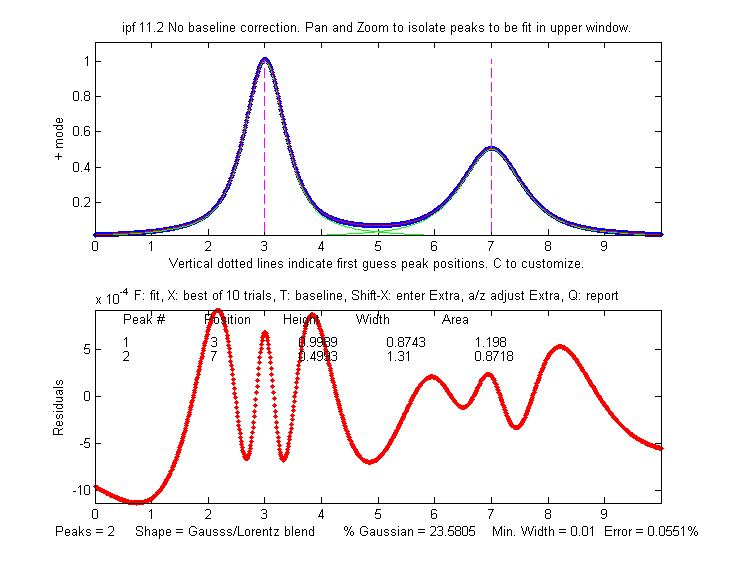
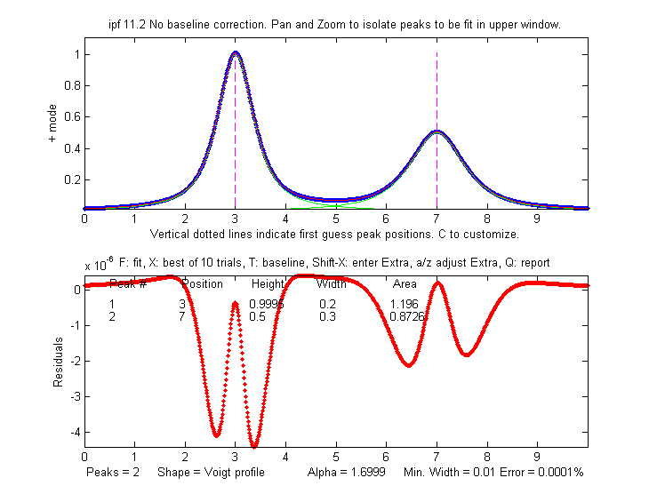
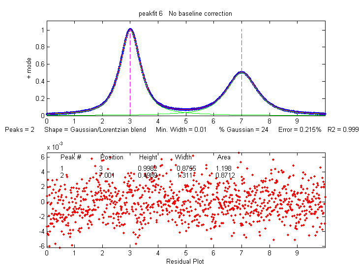
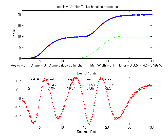
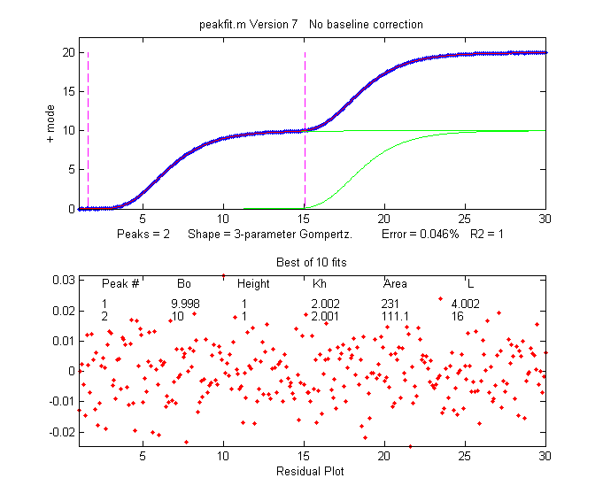
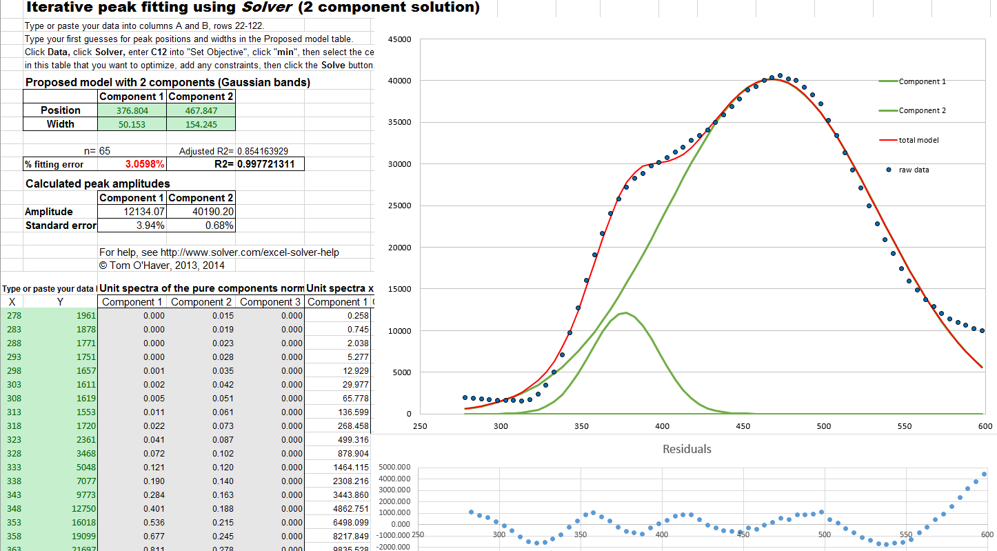
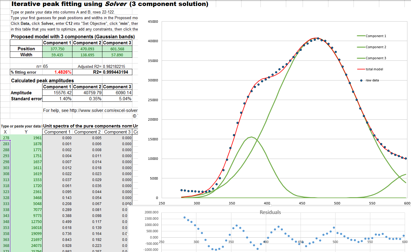
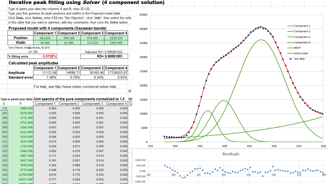
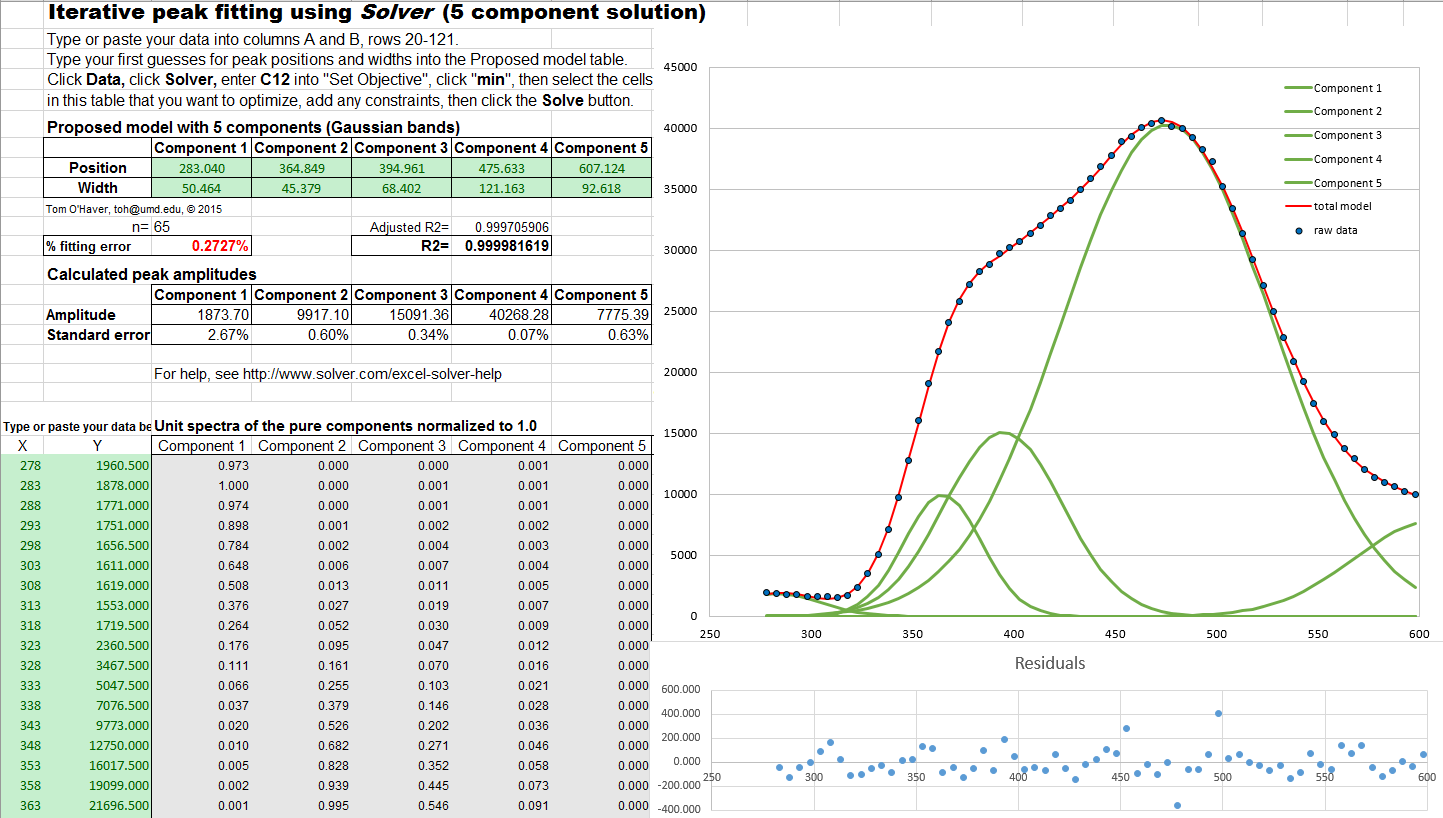
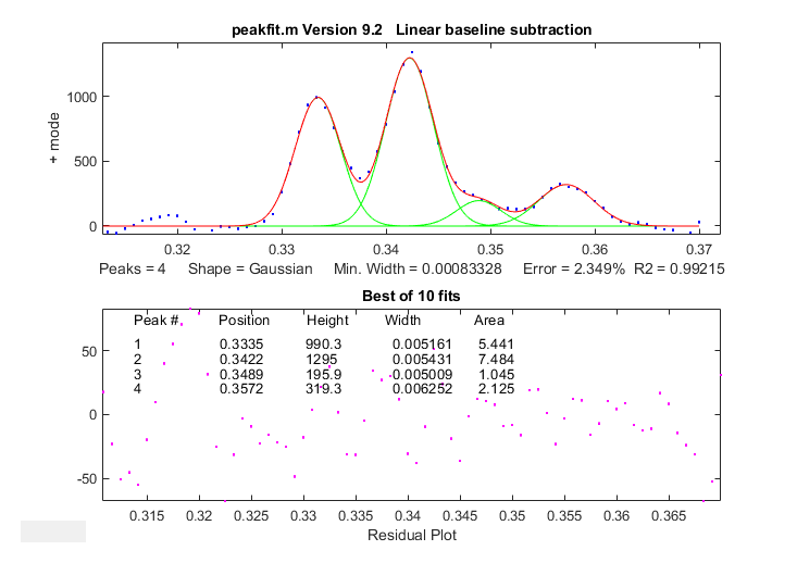
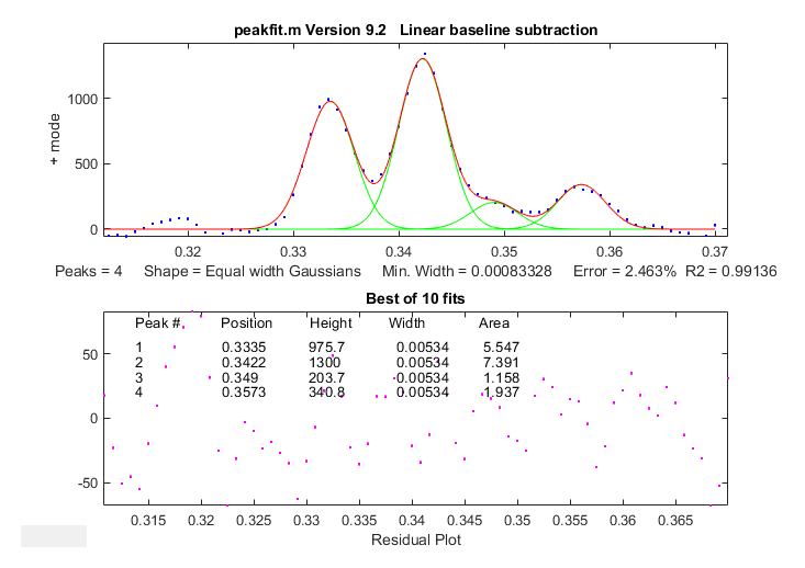
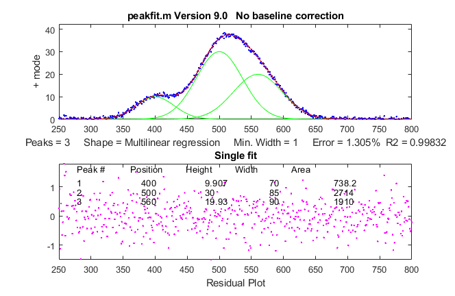
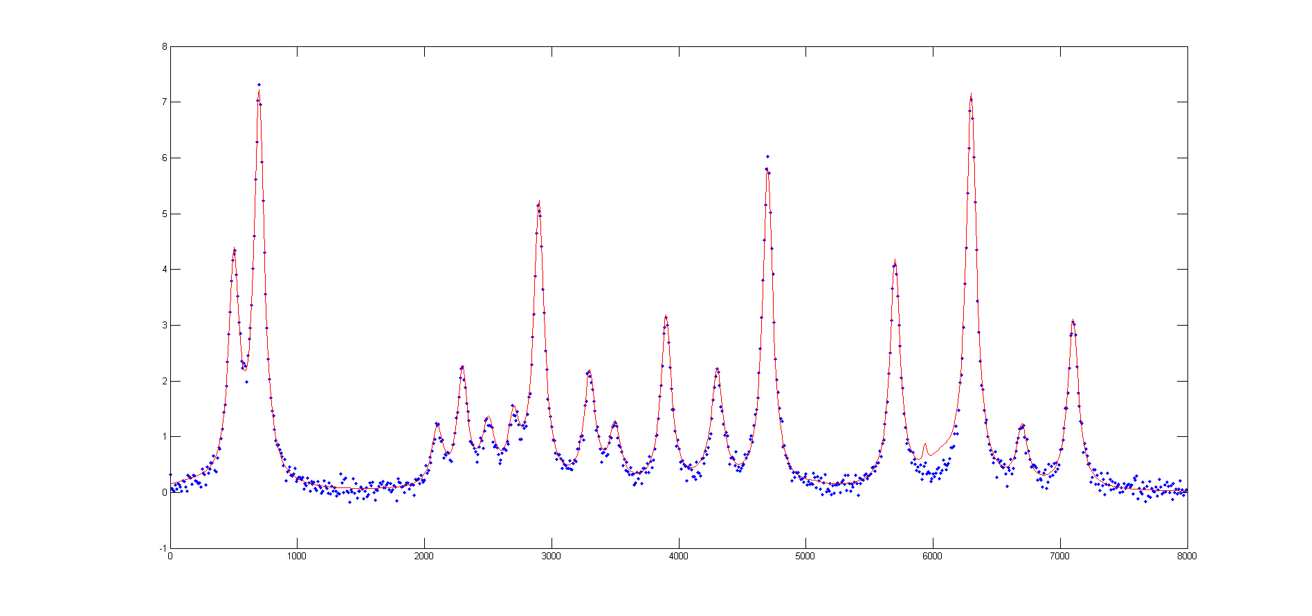
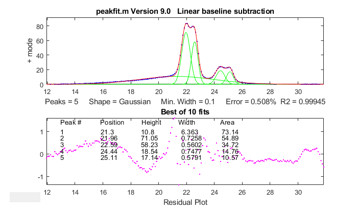
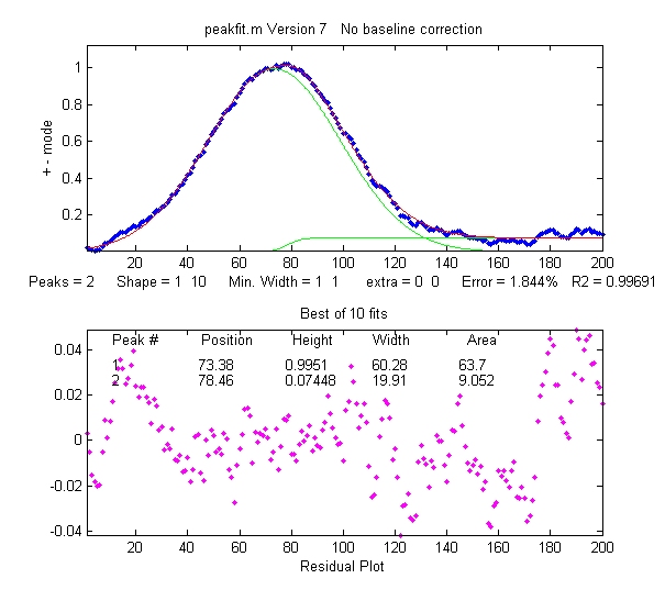
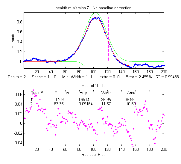
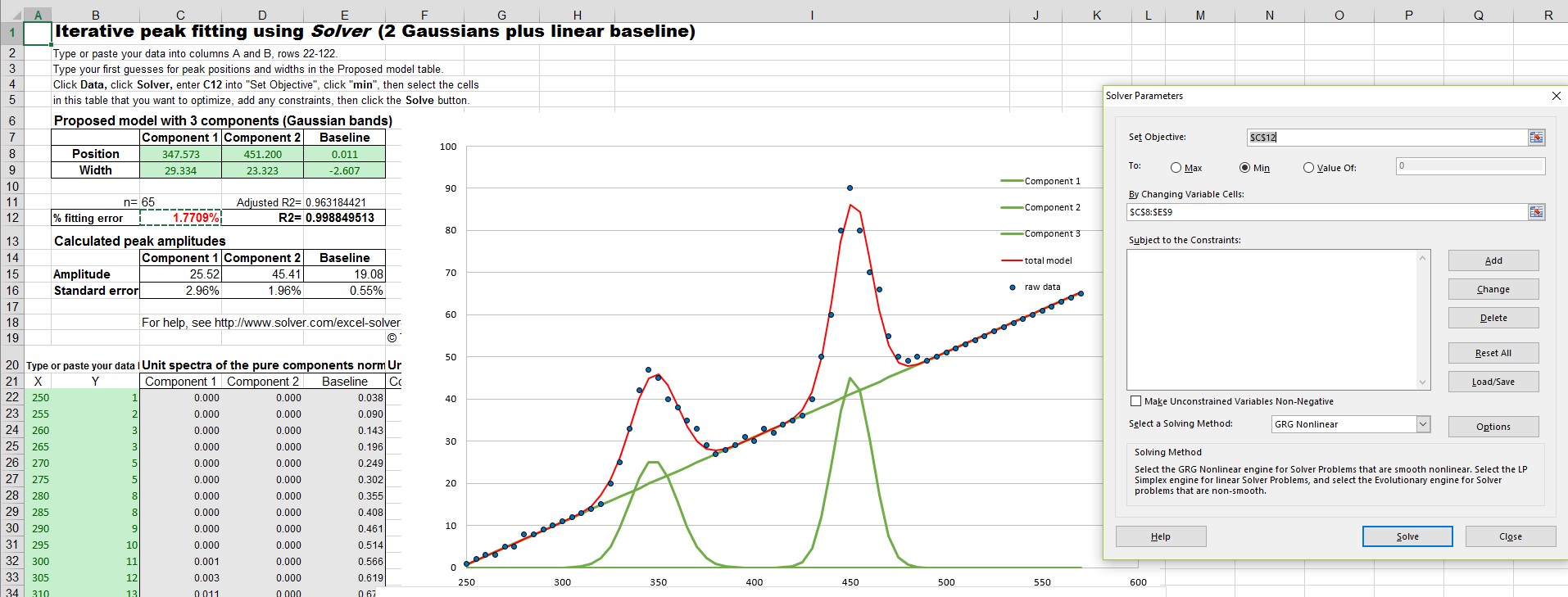
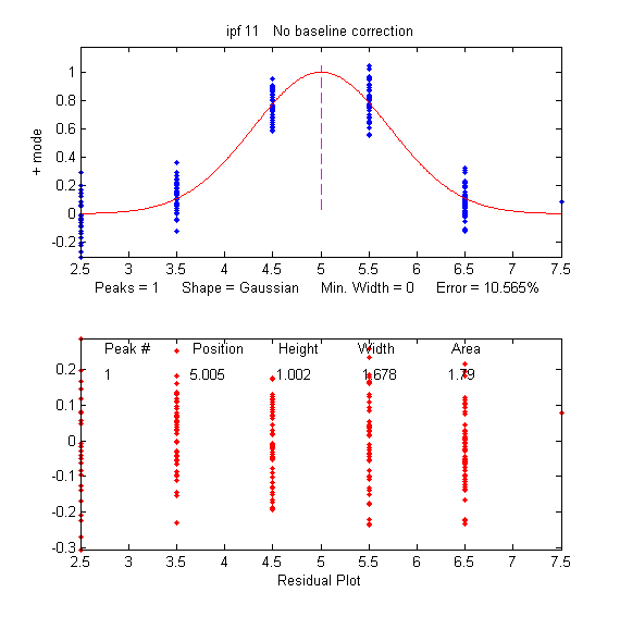
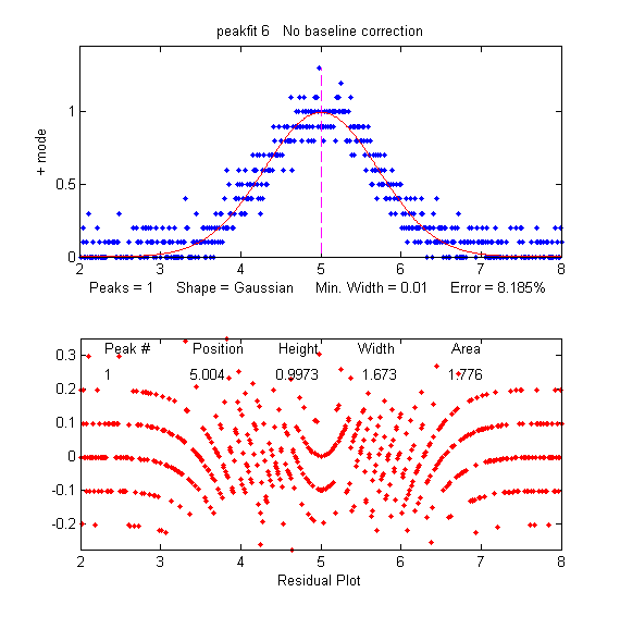
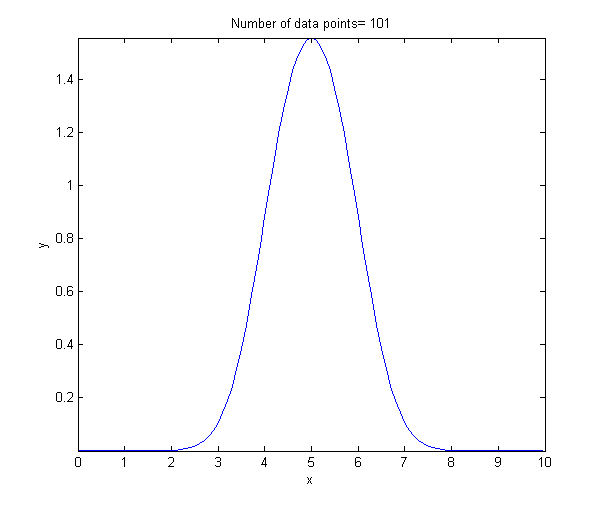
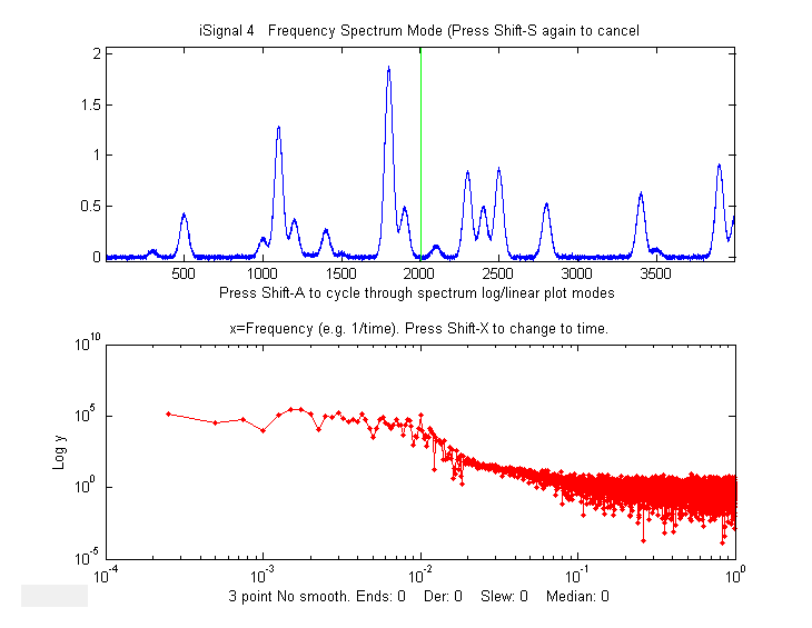
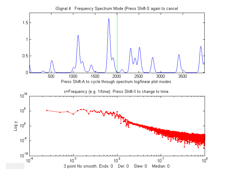